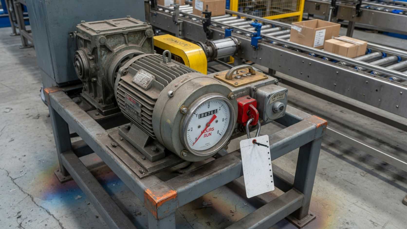
On the floor, “MTBF” often arrives as one number and a twisted question: “so how often does it actually fail?” The figure can help. Read as a countdown for one motor or gearbox, that question is not what the indicator answers.
Mean Time Between Failures summarizes, for a declared population and window, accumulated exposure divided by the failures that meet the counting rule. NIST/SEMATECH estimates it as total operating time over total failures under a constant-rate model. NIST e-Handbook, §8.4.5.1
NASA illustrates the same ratio with operating hours and observed failures in its reliability-centered maintenance guide. NASA RCM Guide
This page is not a manufacturer catalog sheet and not a Weibull tutorial. Formula-level explainers already exist as plant resources for MTBF definition and interpretation. The boundary here is narrower: which question the number answers in the corridor, which hours and failures must stay written down, and when the mean stops being comparable or stops being enough.
The numerical examples are hypothetical or taken from the cited sources. They do not describe your plant or an ROI. WizeeMind gathers operational evidence with source, time, and asset limits; it does not calculate the plant’s official MTBF. If the next step is human, talk to us.
What question MTBF actually answers
In the usual plant reading, MTBF says how many exposure hours were observed for each qualified failure in a defined set. It does not say “when will this unit fail?” and it does not say “is it safe to run until that figure?”
NIST states the estimate under the HPP/exponential model: estimated MTBF = total system (or unit) operation time ÷ total number of failures. NIST e-Handbook, §8.4.5.1
NASA, in §5.5.5.2, writes the failure rate as number of failures over total operating hours and inverts that rate to obtain MTBF under the exponential assumption used in the example. NASA RCM Guide
The result is an average of what was observed. If five units contribute hours and failures to the same ledger, you describe the set, not the fate of unit number three.
Siemens, in a power-supply equipment manual, puts that limit in writing: the MTBF number is a statistical indication of failure probability and does not necessarily represent the useful life of the product. Siemens 8US Manual, §11
One detail of the constant-rate assumption gets lost in many meetings. NASA notes that, with a constant rate, reliability at the mean life is about 0.37: roughly a 37% chance of surviving that mean life without failure. NASA RCM Guide, §5.5.5.1 Reading “761 h MTBF” as “it fails at 761 h” collides with that reading.
On the floor, the useful question is narrower: “in this population, with these hours and this failure rule, what mean do we observe?” That supports trends, comparable periods, and the talk with production about exposure. It does not replace analysis of a specific failure mode, and it does not decide lockout for you.
SAE JA1011 frames reliability-centered maintenance as evaluation criteria for organizations that manage physical assets or systems. SAE JA1011_202411 MTBF can feed that conversation. By itself it is not a complete RCM process and not a strategy verdict.
When someone asks for “the MTBF of fan 12,” they often mix three requests: the history of that unit, the family mean, and a prediction. Keep them separate. The history can list intervals between events. The family mean is the aggregated ratio. A prediction needs another model and other evidence. Bundle all three under the same acronym and an honest indicator turns into a false countdown.
For the rate tied to the ratio, plant resources on failure rate organize the inverse reading. Here it is enough not to treat MTBF as an individual clock.
Running hours versus calendar hours
The numerator decides the question. Running hours between failures give running hours per observed failure. Calendar hours between failures give another quantity: elapsed time per event, not operating exposure.
NASA’s example uses “Total Operating Hours” and failures in operating hours, not calendar days of the month. NASA RCM Guide, tables 5-6 and 5-7 NIST speaks of “Total System(s) operation time” in the MTBF estimator. NIST e-Handbook, §8.4.5.1
Picture a hypothetical case. Asset A accumulates 360 running hours in a month and records one qualified failure. Asset B accumulates 180 hours and also one failure. With running hours, the ratios are 360 h and 180 h per failure. If someone forces 720 calendar hours for both, the results look equal and answer a different question. The numbers are invented to show the numerator effect; they do not describe a real plant.
The hour-run meter does not always win by default. It fits when the question is in-service reliability. Equipment that barely starts can accumulate few failures and few hours while the calendar keeps moving. A three-shift asset accumulates exposure faster. Comparing them on the same wall clock distorts the mean.
Also declare what counts as running. Productive hours? Energized hours? Hours above a minimum speed? Without that note, two shifts can fill the same CMMS field with different criteria.
NIST distinguishes repairable systems (where the interest is failure occurrence rate or repair rate) from non-repairable populations (where life models speak to first failure). NIST e-Handbook, §8.1.2.1
In an industrial plant most process assets are repairable: they return to service. That is why you usually measure operating exposure between events, not only days between work orders.
Siemens publishes MTBF tables tied to current and ambient temperature, and cites SN 29500 / IEC 61709 and MIL HDBK 217F methods. Siemens 8US Manual, §11
Those catalog conditions are not your switchroom. They work as a contrast: even the manufacturer anchors the number to a thermal and load profile. Your plant report should anchor its own number to effective hours and the regime you actually observed.
A minimal card can carry two clocks at once: window dates (calendar) and accumulated running hours (exposure). Then the reader knows the period and the base of the ratio. If you only have open and close dates on a work order, do not call the difference “running hours” unless you can show the asset was operating.
When you produce the number for management, write the full unit: “running hours per qualified failure,” not only “800 hours.” That short label stops someone reading it as calendar days until the next breakdown. Availability and repair-time pieces belong in a separate frame; do not mix those clocks into the MTBF cell.
What counts as a failure
The denominator looks simple until you open the CMMS. An alarm, a stop, a corrective order, and a duplicate notice can describe the same incident or four different things. MTBF is readable only if the inclusion rule stays written.
NASA states that MTBF should be calculated from machinery history in the CMMS and other sources (operator logs, parts use, contractors). NASA RCM Guide, §5.5.5.1 It does not impose your local taxonomy. It does remind you that the data comes from records, not corridor intuition.
NIST estimates MTBF with the total number of failures in the observation period. NIST e-Handbook, §8.4.5.1 If your extract counts “all corrective orders” and another plant counts “only loss of required function,” the ratios do not speak the same language even when both say MTBF.
An operational rule can answer, in writing, concrete questions:
- Which event loses the required function?
- Do you count every notice or each consolidated incident?
- How are duplicates and reopenings handled?
- Do test-detected failures enter, or only in-service events?
- What happens to events still open when the window closes?
Do not copy someone else’s list as law. Adapt the rule to your code system and keep it visible next to the number. If the rule changes after a CMMS migration, note the change date. A “before/after” series can mix equipment behavior with recording behavior.
NASA distinguishes MTBF (tied to failures) from MTBM (mean time between maintenance), which includes corrective and preventive actions. NASA RCM Guide, §14.3 If you put preventives in the denominator and still call the result MTBF, you have changed indicators. Operational availability in that section is expressed with MTBM and mean downtime, not by swapping labels for convenience.
HSE reminds you that maintenance of work equipment must be planned and carried out safely, and that an effective programme makes equipment more reliable; it also warns that unsafe maintenance has caused serious injuries. HSE, Maintenance of work equipment It does not define your failure code. It does mark another boundary: misclassifying an event in the indicator does not authorize improvising the repair work.
Hypothetical example: during an invented window there are six corrective orders and two preventives. An MTBF count with the six failures is not interchangeable with an MTBM count with eight actions. They answer different tallies. Label them separately.
If the debate is predictive versus preventive or corrective, strategy choice is not decided by the MTBF denominator alone. That matrix sits in predictive, preventive, or corrective maintenance. The point here is shorter: without a failure rule, the mean is an orphan number.
Why a “good” mean can hide failure clusters
A mean compresses the story. Two populations can share the same MTBF and distribute failures very differently: some spaced out, others in clusters. The ratio does not show that dispersion.
NIST describes the bathtub curve: an early period of high, decreasing rate, a more or less flat intrinsic stretch, and, if use continues long enough, wearout with a rising rate. NIST e-Handbook, §8.1.2.4
NASA, when it assumes exponential in its example, places the calculation in a relatively constant-rate regime for a mature system, outside infant mortality and before wearout. NASA RCM Guide, §5.5.5.2
If failures cluster after format changes, cold starts, or a specific campaign, the quarter mean can look “acceptable” while production carries three bad weeks. The indicator is not lying; it is summarizing. Anyone who only watches the summary misses the cluster.
With few failures, the point estimate misleads more than it seems. NIST gives an example with 800 hours of operation and 2 failures: estimated MTBF of 400 h, and a 90% confidence interval between 127 and 2,251 h. NIST e-Handbook, §8.4.5.1 With r = 0, only a one-sided lower bound exists. A “nice” mean with two events does not close the debate.
Siemens illustrates the population reading with a catalog numerical example: an MTBF of 1,000,000 h means, statistically, that one unit will fail every 100 h if 10,000 units are installed. It does not say whether the failed unit had 50,000 h or only 100 h. Siemens 8US Manual, §11
Translate that to the plant: a high family mean can sit next to one concrete asset that already has its third event this month.
When you suspect clusters, drop to the interval list instead of arguing only the average. Sort dates, shifts, product, running state, and recent work. Downtime analysis with operational evidence helps you avoid closing the story with the most convenient code; see downtime analysis with operational evidence.
Douglas Thomas, in NIST AMS 100-18, examines maintenance costs and losses (direct, downtime, defects) and the need for data to separate them across approaches. NIST AMS 100-18 A “good” MTBF does not prove by itself that downtime costs fell. It can hide an expensive cluster offset by long quiet stretches on other assets in the same bag.
Next to the period MTBF, publish the failure count, the accumulated hours, and, if the tally is small, an uncertainty note. You do not need a statistics tutorial on the board. You do need to stop five unevenly spaced events from being sold as uniform stability.
When you can compare two MTBF figures
Comparing two MTBF values without a card is the usual meeting shortcut. Matching numbers do not prove matching conditions. Different numbers alone also do not prove that one line is “better.”
Before you put them in the same table, align at least population (which identifiers enter and which are excluded), hour type (running, energized, calendar, or other), window (dates and regime), failure rule with duplicate handling, and whether the set is repairable and what was done after each event.
Under the model described, NIST estimates MTBF the same way with censored or complete data, but the confidence interval depends on the number of failures. NIST e-Handbook, §8.4.5.1 Comparing a period with 2 failures against another with 40 without looking at uncertainty is precision theater.
NASA’s teaching example uses 3,805 total hours and 5 failures: 761 h MTBF under the exponential assumption. NASA RCM Guide, §5.5.5.2 If you quote “761” without the 3,805 hours, the five failures, and the assumption, you lose the context the guide itself keeps next to the number.
Siemens shows how the catalog figure changes when temperature, current, and method change (IEC 61709 / SN 29500 versus MIL HDBK 217F with different environmental classes). Siemens 8US Manual, §11 That sensitivity of conditions works as a plant warning: if period B added a third shift or switched to an abrasive product, do not compare it blindly with period A.
Hypothetical false-equivalence example: set A with 2,400 h and 4 failures (600 h/failure); set B with 3,600 h and 6 failures (also 600 h/failure). The ratios match. Without knowing load, group composition, and recording rule, the match does not prove equivalent reliability.
SAE JA1011 offers criteria for evaluating RCM processes in organizations that manage physical assets. SAE JA1011_202411 Comparing MTBF can be an input to that management. It does not replace defining functions, failure modes, and consequences.
When the comparison crosses manufacturer and plant, keep the boundary clear: the catalog speaks to product and declared conditions; the history speaks to what was recorded in your window. A gap between the two does not, by itself, date the next failure of one unit. Formula-level MTBF plant resources draw that same line without turning the catalog into a calendar.
When the comparison is internal (line 1 versus line 2, or quarter versus quarter), write down what changed in data capture. A “better MTBF” after you trained technicians to consolidate notices can be a denominator change, not a mechanical one.
Limits: not a next-failure timer and not a safety certificate
MTBF does not work as a timer. It also does not certify that an asset is safe, prove that a maintenance strategy worked, or replace lockout, competence, or local procedures. HSE separates operational reliability from the duty to keep work equipment in a safe working condition. HSE, Maintenance of work equipment
NASA ties its numerical example to the exponential distribution assumption and a relatively constant rate in normal operation of a mature system. NASA RCM Guide, §5.5.5.2 If the rate changes with age, load, or environment, that example is not a forecast of the next breakdown.
NIST places most of the useful life, with luck, in the flat zone of the bathtub, and also documents infant mortality and wearout. NIST e-Handbook, §8.1.2.4
Siemens states that MTBF does not necessarily represent product life and that, from the aggregated number, you cannot tell whether the failed unit had many hours or few. Siemens 8US Manual, §11 That catalog limitation holds equally for a plant mean.
HSE requires work equipment to be maintained in an efficient state, in efficient order and in good repair, and notes that undiagnosed faults add hazards. HSE, Maintenance of work equipment A high MTBF does not prove that duty was met. A low one also does not authorize improvising isolation or skipping competent staff. HSE guidance is for Great Britain; your plant follows the local obligations that apply.
Douglas Thomas frames the economic value of advanced maintenance as a problem of costs and losses that needs data (direct maintenance, downtime, lost sales, rework, defects) and separation across techniques. NIST AMS 100-18 MTBF can enter the file. It does not close the business case or the balance among reactive, preventive, and predictive work.
Explicit limits of this page:
- Do not use MTBF as an expiry date for one concrete asset.
- Do not use it as a safety certificate.
- Do not compare figures without aligning population, hours, window, and failure rule.
- Do not confuse MTBF with MTBM or with availability.
- Do not replace evidence of a failure mode with the bag average.
Read as an observed mean with a card, the figure stays useful. You see whether exposure per failure moves across comparable periods. You catch criterion changes in numerator or denominator. You open the event list when the mean and the floor disagree. Past that, do not ask more of it than it can carry.
If you need to choose a task by failure mode, go back to the matrix in predictive, preventive, or corrective maintenance. If you need to rebuild a stop, use evidence with window and source. MTBF summarizes; it does not investigate. WizeeMind does not calculate official MTBF. To gather the trail with source and asset limits, talk to us.
Frequently asked questions
Does MTBF say when this piece of equipment will fail?
No. Observed MTBF is a mean for a declared population and window; it does not fix the failure date of one unit. NIST estimates MTBF as total operating time over total failures under the constant-rate model. NIST e-Handbook, §8.4.5.1
Siemens adds that the number is a statistical indication and not necessarily product life. Siemens 8US Manual, §11
Calendar hours or running hours?
For operational reliability, use running hours (or another effective exposure). Calendar hours answer a different question. NASA and NIST build the estimator with operating hours, not with the mere passage of the month. NASA RCM Guide NIST e-Handbook, §8.4.5.1
Does a high MTBF prove the asset is reliable or safe?
No. A high MTBF summarizes an observed ratio; it does not certify safety or replace competent maintenance of the equipment. HSE ties safety to planned, competent maintenance of work equipment, not to a failure average. HSE, Maintenance of work equipment NIST reminds you that the rate may not stay constant across the whole life. NIST e-Handbook, bathtub
What must sit next to the figure so you can read it?
At minimum: population, window, hour type, and the rule for what counts as a failure, plus how duplicates and exclusions are handled. NASA keeps total hours, failure count, and model assumption next to its example. NASA RCM Guide, §5.5.5.2
Siemens anchors its tables to current, temperature, and method. Siemens 8US Manual, §11
When can you compare two MTBF figures?
When population, exposure, window, and failure rule are compatible. If any of those fields differ, leave the comparison open. NIST confidence intervals show how wide the estimate becomes with few failures. NIST e-Handbook, §8.4.5.1
SAE JA1011 frames responsible asset management; it does not turn two orphan figures into a benchmark. SAE JA1011_202411
Does WizeeMind calculate the plant’s official MTBF?
No. WizeeMind gathers operational evidence with source, time, and asset limits; it does not calculate the plant’s official MTBF. An official MTBF needs local definitions of population, hours, failures, and window, plus the data chain that supports them. NIST AMS 100-18 stresses the need for data to estimate maintenance costs and losses; an external panel does not certify the indicator. NIST AMS 100-18
Sources
- NASA: Reliability-Centered Maintenance Guide (PDF)
- NIST/SEMATECH e-Handbook: Constant repair rate (HPP/exponential) model
- NIST/SEMATECH e-Handbook: Bathtub curve
- NIST/SEMATECH e-Handbook: Repairable systems and lifetime models
- NIST AMS 100-18: Costs and Benefits of Advanced Maintenance in Manufacturing
- HSE: Maintenance of work equipment
- SAE JA1011_202411: Evaluation Criteria for RCM Processes
- Siemens: Power supply unit 8US2830-2BE01 Equipment Manual (MTBF / IEC 61709)